Monte Carlo Methods in Finance¶

The result obtained using the analytical formula in the previous exercise is $V_A=11.5442802271$ and the option delta is $\Delta_A=0.6737355117348961$

An $\alpha$-significant confidence interval is given by

\begin{equation} \bar{X} \pm \mathcal{Z}_{\alpha/2}\frac{s}{\sqrt{n}} \end{equation}

where $\frac{s}{\sqrt{n}}$ is the standard error. Throughout the report I will use $\alpha = 0.01$ when a confidence interval is required, otherwise the standard error is reported.

We find that with 1,000,000 samples we get within a few hundreds error of the actual value:

$$ V_{MC} = 11.54408186\pm0.0406364867056 $$

Convergence¶

We investigate the point estimate for the option value and confidence interval for increasing number of values.

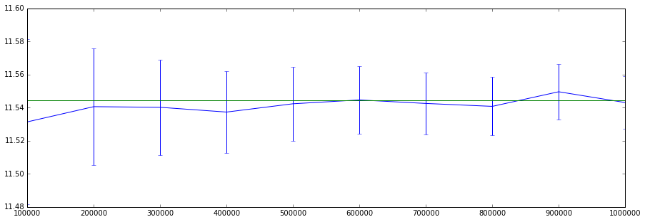We see the estimate converge on the analytical result. Choosing a different seed leads to errors of the same magnitude but different realisation. We see that the standard error decreases as the number of samples is increased.

Compared to other techniques such as the binomial tree we now have a probabilistic method whereas the binomial tree method is deterministic, and this method requires more computation time and memory in order to get the same number of significant digits (verified by the analytical result).

Discretisation¶

\begin{equation} S_t = S_0 e^{(r - \frac{1}{2}\sigma^2)t + \sigma \sqrt{T}Z_t} \end{equation}

The process chosen to model the underlying is $$ dS = rSdt + \sigma S dZ $$

We then discretise the process into $n=\frac{T}{\Delta t}$ time steps.

Using the forward Euler method we obtain the discretisation

$$ S_{n+1}=S_n + rS_n\Delta t + \sigma S_n\phi\sqrt{\Delta t}) $$

This requires that we simulate the process at every timestep in order to compute the result.

If the coefficients $r, \sigma$ are constant however we can integrate over time in order to obtain equation 2 which we will do now.

We convert the equation to log space

$$ L = \log{S} $$

Now, by applying Ito's lemma to $L$ we obtain:

$$ dL = \frac{dL}{dS}dS + \frac{1}{2}\frac{d^2L}{dS^2}\sigma^2 S^2 dt $$$$ dL = \frac{1}{S}(rSdt + \sigma S dZ) + \frac{1}{2}\frac{1}{-S^2}\sigma^2 S^2 dt $$$$ dL = (rdt + \sigma dZ) - \frac{1}{2}\sigma^2dt $$$$ dL = (r - \frac{1}{2}\sigma^2)dt + \sigma dZ $$$$ L = c + \int_0^T(r - \frac{1}{2}\sigma^2) dt + \int_0^T \sigma dZ $$

We argue here that the randomness is caused by the Wiener process term $\sigma dZ$. Now, for pricing models where only the value at the end matters we might argue that a sample might be realised by taking a single random value $Z_t$ and scaling it by $\sigma \sqrt{T}$, since the process accumulates a variance of $T$ and in this logspace transform is normal-distributed. This allows us to generate the end prices without simulating the whole path of the assets, and is therefore faster to compute.

$$ L_T = c + (r - \frac{1}{2}\sigma^2)T + \sigma \sqrt{T}Z_t $$

When we take the constant of integration $c = log(S_0)$ and exponentiate the remainder:

$$ S_t = S_0 e^{(r - \frac{1}{2}\sigma^2)t + \sigma \sqrt{T}Z_t} $$

Equation 2 allows us to jump to maturity immediately and is therefore computationally less intensive.

Error sensitivity¶

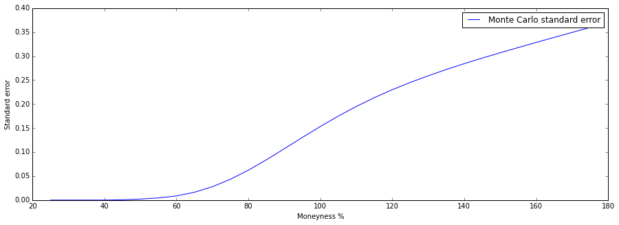Varying the moneyness ($\frac{S}{K}$) of the option. We see that the standard error is increasing in the moneyness. The shape of the curve reminds us somewhat of the option $\Delta=\frac{\partial V}{\partial S}$: when the option is far out of the money, the standard error is close to zero, exactly like the delta. The error is close to zero because the option has a minimum value of 0. When the option is at the money both the standard error and the delta change the fastest. Whereas the delta approaches $1$ when the option is far in the money, the standard error is shown to to be increasing. This is because the option value changes almost 1-to-1 with the increase of the spot price (the delta is one) and this scales the standard error up along with it.

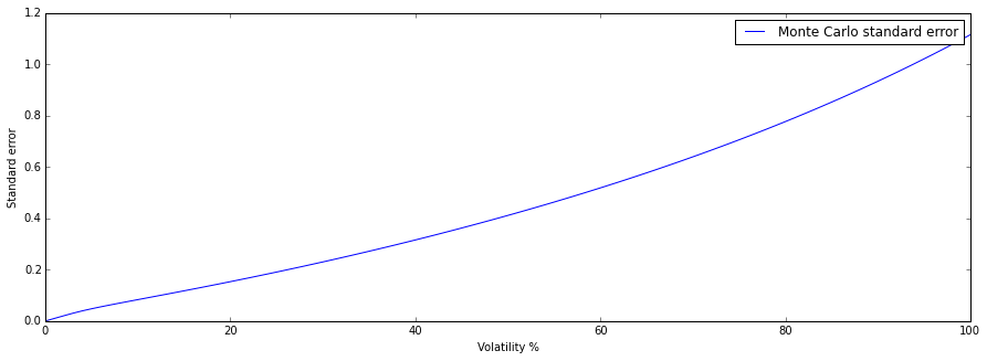Varying the moneyness ($\frac{S}{K}$) of the option. We see that the standard error is increasing in the volatility. Since the value of the option is increasing in the volatility, we know that the standard error will increase when the volatility increased. When the volatility is close to 0, for this spot $S=100$ and strike $K=99$ the option value is close to zero.

Estimation of Sensitivities in MC¶

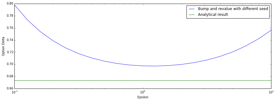Estimates of the option delta with different seeds. In this instance we find a minimum around $\epsilon\approx 1$. This value is arbitrary since it depends on the number of samples simulated, but we will use it in our explanation of the errors on both side: when the epsilon value is chosen smaller than this minimum, the error between the two random point estimates starts to dominate the epsilon value. When epsilon is chosen larger, the finite difference is too large to accurately estimate the first derivative with respect to the underlying (the delta). The standard errors are displayed in the following plot in order to improve the visualisation.

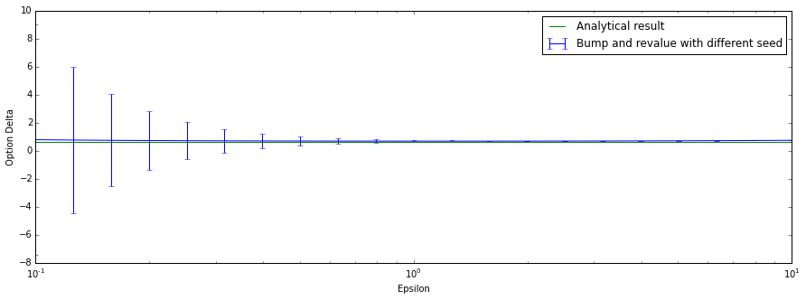The same expirement but now with the standard error added. We see that for small epsilon values the standard error becomes very large: this is evidence that the method becomes unstable due to the error between the point estimates with random seeds dominating the epsilon value.

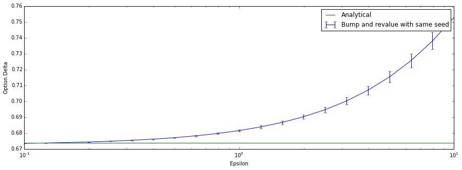Using the same seeds for both point estimates. We see that not only does the method converge beautifully on the target, the standard error also decreases as we choose a smaller epsilon. Note that this method still becomes unstable when we choose epsilon very close to the machine epsilon (machine precision number) due to numerical errors.

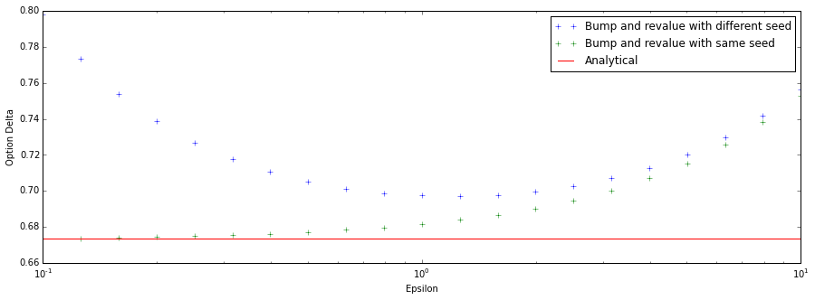In this combined chart we see that the error of the difference between the two randomly chosen point estimates only exists when choosing a different seed: as epsilon increases both methods revert to the same error due to the large interval.

The payoff function of the binary Cash-or-nothing call option is $1$ if the spot price is larger than the strike at maturity, $0$ otherwise.

This can be modeled using:

\begin{equation} V = \mathcal{H}(S-K) \end{equation}

where $\mathcal{H}$ is the discrete version of the Heaviside function $\mathcal{H}(x) = \left\{ \begin{array}{lr} 0 & : x \leq 0\\ 1 & : x > 0 \end{array} \right.$. The function is discontinuous at $x=0$.

I use an analytical solution for both the value and delta for binary options (see code).

We find that the standard error is not decreasing and is for these different choices of $\epsilon$ almost constant. Even for averages of many point estimates the error is still relatively high $\frac{\sigma}{\sqrt{n}}\approx 0.00180496$. Note that the estimate is still relatively unstable, even for an average of several runs each with different seeds.

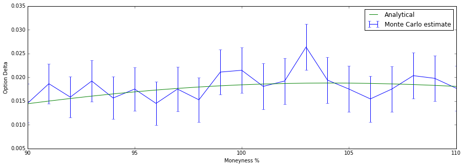Estimating the delta of the binary option for different moneyness. We see that the method is somewhat unstable and jumps around when some of the parameters are changed only slightly. This is due to the fact that when the same paths are shifted slightly (for example choosing a different starting price), all of a sudden a large bundle of paths can have a radically different payoff when they end up on the other side of the strike price.

The method I will be using is smoothing using a sigmoid function of the following form:

\begin{equation} S(x) = \frac{1}{1 + e^{-kx}} \end{equation}

Here $k$ is a parameter that we can choose in order to change the steepness of the curve. The function has many advantages. The main reason we use this function for smoothing is that it is continuous. It is also fast to compute. When we choose $k$ large enough, this function converges on the actual Heaviside function.

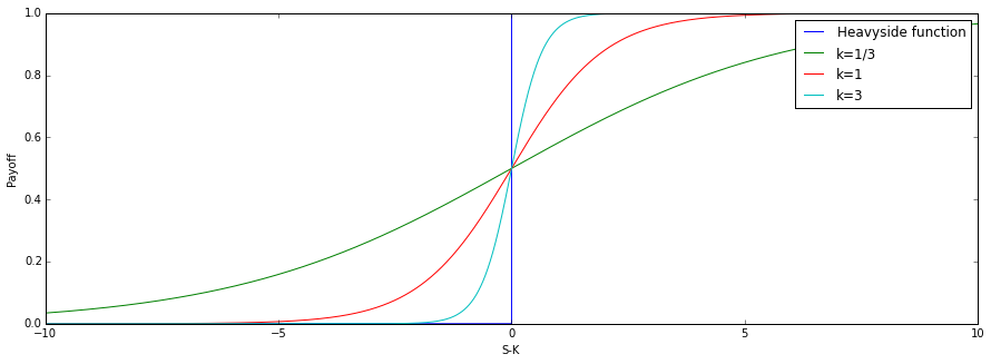The payoff function for the binary cash-or-nothing call option (displayed as the Heaviside function with a step plot, note that there is a discontinuity) and 3 choices for the steepness of the smoothed curve.

We are now to choose $k$. We have on one hand consider that choosing a large $k$ gives us a function closer to the actual payoff function. But this gives us the problems of a bundle of paths having a radically different payoff when shifted only slightly. Choosing a small value gives us a smoother function but will give us a more incorrect payoff function: imagine a very small value of $k$, the payoff function is nearly $\frac{1}{2}$ everywhere. This option would have the same value for all values of moneyness and this is not what we want. The choice for $k$ depends therefore mostly on what we can do in programming (my Python runtime throws exceptions when the exponent gets too large due to numerical errors) and most importantly our choices for parameters to the model. We make a quick plot for $k$ and the relative error to the analytic result and we find:

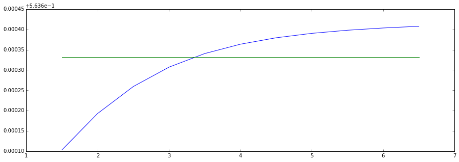For this set of parameters, $k=3.5$ seems to be optimal. On the x-axis the choice for $k$, and on the y-axis the relative error.

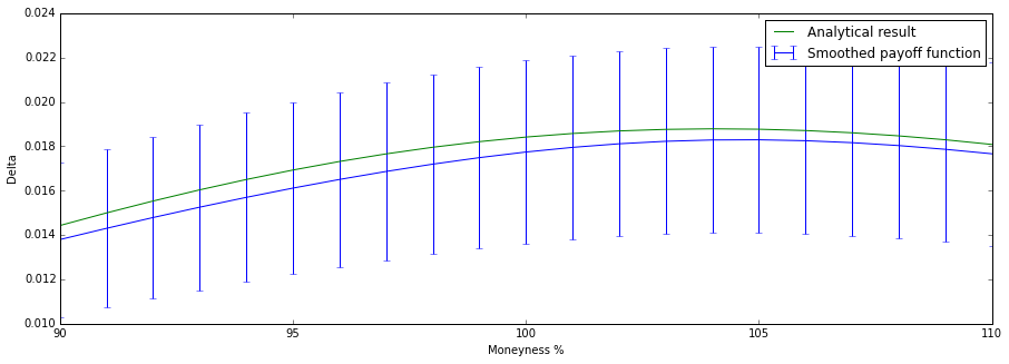We see that the Monte Carlo result is smaller for every test. This is due to simple chance (in essence the choice of the seed for the RNG. I found that by increasing the number of samples the estimated delta converges on the analytical result.)

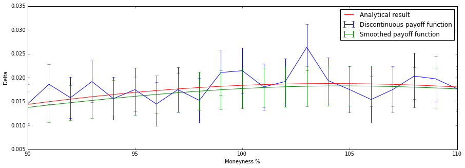In this combined chart we see that the smoothing method offers not only a better estimate and better stability, but also a smaller standard error.

Variance Reduction¶

Variance Reduction by Antithetic Variables¶

By the Central Limit Theorem, the arithmetic mean of independently and identically distributed random variables is normally distributed. More formally, let $X$ a series of $n$ random variables then as $n \to \infty$

$$ \frac{(\sum_{i=1}^{n}X_i) - n E[X_1]}{\sqrt{n}\sigma } \rightarrow \mathcal{N}(0, 1) $$

The standard error is given by $\frac{\sigma}{\sqrt{n}}$. We assume $\sigma$ to be a known, finite constant so the error converges only by:

$$ \mathcal{O}(\frac{1}{\sqrt{n}}) $$

In other words, the error becomes smaller as the number of samples is increased but rather weakly (note the square root term).

Antithetic Variates is a method to reduce variance. The method works in essence by taking for every simulated instance of a stochastic process $X = [x_1, x_2 \ldots x_n]$ also taking the antithetic path $X' = [-x_1, -x_2 \ldots -x_n]$. This guarantees that the covariance between these paths is negative. We will see this formalised below.

Note that in order to compare methods, we should compare $n$ samples of plain Monte Carlo with $n/2$ samples of the Antithetic Variates method since we are creating two paths every time.

Expression for the variance of the antithetic variables point estimate¶

The variance is given by:

$$ var(X \cup Y) = \frac{var(X) + var(Y) + 2covariance(X,Y)}{4} $$

When we take the antithetical values of X for Y the covariance becomes negative. This decreases the variance of the whole set of paths.

$$V_{AV} = 11.554704079951877 \pm 0.010527588002357402$$$$V_{MC} = 11.544081860012135 \pm 0.01581276511238136$$

We see here that using antithetic variables the standard error is much smaller than using the plain Monte Carlo method.

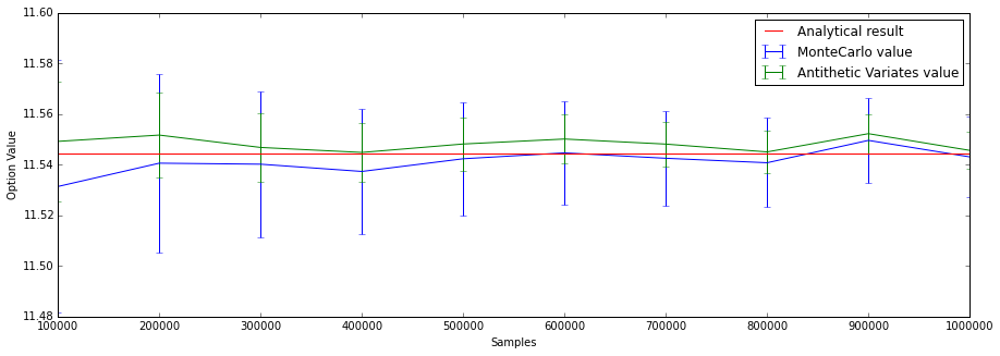Using the antithetic variates we get a symmetric distribution of random terms. This changes the bias in the plain Monte Carlo method. We see a much smaller standard error.

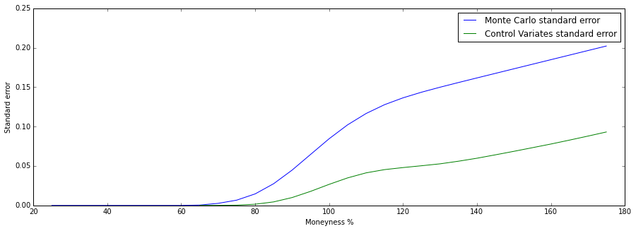
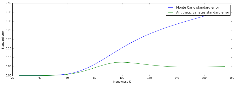\caption{Interestingly we see that the standard error for Antithetic Variates is a much smaller and doesn't seem to scale as much for in the money options. It is likely that AV performs much better for options far in- or out-the-money due to the fact that the price now depends on a distribution that is guaranteed symmetric (we chose the antithetic paths).

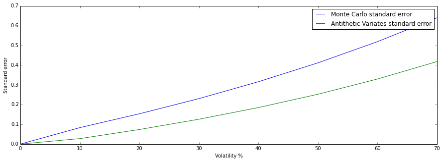The standard error scales similarly in the volatility for the Antithetic Variates method.

Variance Reduction by Control Variates¶

We are interested in some value $C_A$ which has Monte Carlo estimate $\hat{C_A}$.

We also have another quantity $B$ that has a more accurate (preferably analytical) value $C_B$ and can also be estimated using a Monte Carlo method using the same paths. It is important that $B$ is somewhat proportional to $A$.

$$ \tilde{C_A} = \hat{C_A} - \beta(\hat{C_B} - C_B) $$

Informally, we can now adjust the weights of the paths by testing them against a known quantity $B$.

The standard error is now

$$ \sigma_A^2 + \beta\sigma_B^2-2\rho\beta\sigma_a\sigma_b $$

This adjustment reduces the variance when

$$ \beta2\sigma_B^2-2\rho\beta\sigma_a\sigma_b < 0 $$

$\beta$ is a parameter that we can choose using information obtained from $A$ and $B$. We choose it as follows: $$ \beta = \frac{\sigma_A}{\sigma_B}\rho $$ \problem{2. Derive an analytical expression for the price of an Asian option that is based on geometric averages.}

The geometric mean is defined as

$$ \tilde{A_N} = \sqrt[n]{\prod_{i=1}^n S_i} $$

We are given the hint that we can express the product as

$$ \sqrt[n]{\prod_{i=1}^n S_i} = \sqrt[n]{\frac{S_n}{S_{n-1}}\frac{S_{n-1}}{S_{n-2}}^2\ldots\frac{S_{1}}{S_{0}}^n S_0^n } $$

Here, every $i$-th term $\frac{S_i}{S_i-1}$ in the product is lognormally distributed , and then $$\log(\frac{S_i}{S_i-1}) \sim \mathcal{N}((r-0.5\sigma^2)\Delta t, \sigma^2 \Delta t)$$

We can take the last $S_0$ term from under the nth-root and use the product/sum identity of the logarithm:

$$ S_0 e^{(1/n)\log(\frac{S_n}{S_{n-1}}) + (2/n)\log(\frac{S_{n-1}}{S_{n-2}}) + \ldots} $$

This is reminiscent of the derivation of the Black-Scholes formula. The drift is now scaled by

$$ \frac{1}{n}\sum_{c=1}^n c = \frac{1}{n}\frac{n^2 - n}{2} $$

and the variance by

$$ \frac{1}{n^2}\sum_{c=1}^n c^2 = \frac{1}{n^2}\frac{n(n+1)(2n+1)}{6} $$

So we end up with a distribution of $\mathcal{N}((r-0.5\sigma^2)\frac{n+1}{2n}T, \sigma^2 \frac{n^2 + 2n + 1}{6{n^2}}T)$

We can enter these in the template (so to speak) of the analytical formula for the call and we obtain:

$$ S_0 e^{-r+(\frac{n+2}{6(n+1)}\sigma2)\frac{T}{2}}\Phi(\frac{(\log{S/K} + \frac{n-1}{6(n+1)}\sigma^2)\frac{T}{2}}{\sqrt{\frac{n+1}{6(n+1)})\frac{T}{2}} \sigma \sqrt{T}}) - K e^{-rT} \Phi(\frac{(\log{S/K} + \sigma^2)\frac{T}{2}}{\sqrt{\frac{n+1}{6(n+1)}\frac{T}{2}} \sigma \sqrt{T}}) $$

\problem{3. Apply the control variates technique for the calculation of the value of the Asian option based on the arithmetic average.}

Plain Monte Carlo $$ 6.4457643521330379 \pm 0.08484775605305271 $$

Using Control Variates:

$$ 6.5684133972768954 \pm 0.02736988012489495 $$

We see that the standard error is much smaller.

\problem{Study the performance of this technique for different parameter settings (number of trails, strike, number of time-point used in the averaging etc).}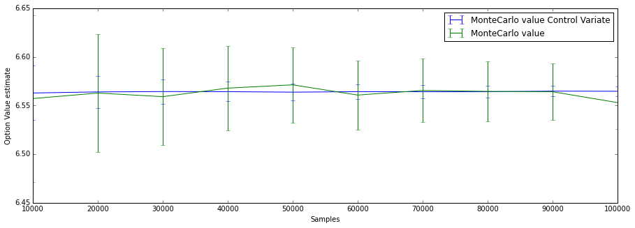

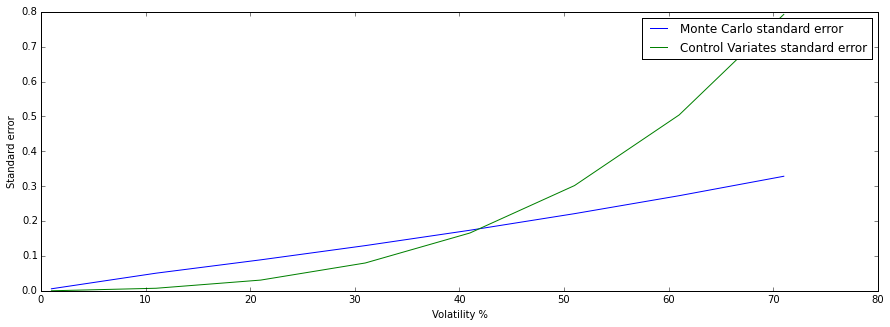Here I plot the standard error by forcing the function to output the CV standard error even if its worse than the plain method. We see here that as the volatility increases, the arithmetic mean and the geometric mean product start to diverge. As a result the standard error worsens in the control variates method, since our adjustment is off.

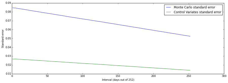
Again the standard error is much smaller.