Fractal Geometry¶

Definition of the Julia set¶

Consider a rational function $f(z) = \frac{P(z)}{Q(z)}$ inside the complex plane $ f : \mathbb{C} \mapsto \mathbb{C} $. There are a finite number of sets $F$ that remain unchanged when transformed by $f$; the sets have the invariance property. The union of the sets in $F$ is dense in the plane. The function $f$ is regular on the sets in $F$: under repeated application of the function, the endpoints of the sequences obtained are a set of cycles. Each of the sets in $F$ have at least one fixpoint. If there is only one such cycle there is an attracting fixpoint, when there are many there is a neutral fixpoint.

The union of the sets in $F$ are the Fatou set of $f$, named after the French mathematician Pierre Fatou (1878-1929). It's complement is the Julia set $J(f)$, after Gaston Julia (1893-1978), also French.

The Julia set is nowhere dense and has the same cardinality as the set of real numbers $\mathbb{R}$: it is uncountable. On this set the iteration of $f$ is repelling. Iteration of $f$ on points outside the set shows deterministic chaos.

Filled-in Julia set¶

The filled-in Julia set for a function $f$ contains the Julia set of $f$ and the interior points. Let $f^{(n)}$ denote the $n$-fold composition of $f$; in essence repeated application, then the filled-in Julia set is defined as follows:

\begin{equation} K(f) = \{z \in \mathbb{C} : f^{(k)}(z)\text{ bounded as }k \rightarrow \infty \} \end{equation}

Because of the repelling property of the critical points of the Julia set, when we repeatedly apply the rational function $f$ for a point $c$ and find that the sequence diverges this means that the point was not part of the Julia set or it's interior.

Fundamental Dichotomy¶

For a subset of $f$ where $f(z) = z^2 +c$, Fatou and Julia proved\cite{fatou} in 1919 that for each $c$ value, the filled in Julia set $K(f)$ is either a Cantor set or a connected set\cite{devaney}.

The Mandelbrot set¶

Complex Polynomial¶

The Mandelbrot set $\mathcal{M}$ is defined by a family of polynomials $P_{c}^{n} : \mathbb{C} \mapsto \mathbb{C}$

\begin{equation}\tag*{Complex Polynomial} P_c^n : z \mapsto z^n + c \end{equation}

where $c$ is a complex parameter and $n$ is the order of the polynomial. The complex plane that $c$ is taken from is referred to as the parameter plane, whereas the values $z_0, z_1, \ldots z_t$ are said to lie in the dynamical plane. For the typical Mandelbrot set the polynomial is quadratic ($n=2$).

Now given a function $f \in P_c^n$ the Mandelbrot set $M$ is defined

\begin{equation} \mathcal{M} = \{ c \in \mathbb{C}: f_c^{(k)}(0) \text{ is bounded as }k \rightarrow 0 \} \tag*{Mandelbrot Set} \end{equation}

The sequence of numbers $z_0, z_1, \ldots z_t$ obtained by the repeated application of $f$ starting with $z_0$ is called the orbit of $z_0$. When $z_0=0$, the next $z_1$ expands to $z_1 = f_c(0) = 0^2 + c = c$. Refer to the element in the orbit at time $t$ as $T^t_n$. We find $T^0_n(c) = 0$, $T^1_n(c) = c$, $T^2_n(c) = c^n + c$ and so on.

In essence: a point $c$ belongs to the Mandelbrot set if, as $t \to \infty$ $T^t_n(c)$ is bounded $\iff$ the filled-in Julia set $K(f)$ is connected for $c$.

Area of the Mandelbrot set¶

Series¶

Ewing and Schober showed\cite{ewing} in 1992 that the area $A$ of the Mandelbrot set can be written exactly as

\begin{equation} A = \pi ( 1 - \sum_{n=1}^{ \infty }nb^2_n ) \end{equation}

where $b_n$ are the coefficients of a Laurent series given by:

$$ b_n = \begin{cases} -\frac{1}{2} & n=0 \\ -\frac{w_{n,n+1}}{n} & otherwise \end{cases} $$$$ w_{n,m} = \begin{cases} 0 & n=0 \\ u_{0, m} + w_{n-1, m} + \sum_{j=0}^{m-2}u_{0,j+1} w_{n-1,m-j-1} & otherwise \end{cases} $$$$ u_{n,k} = \begin{cases} 1 & 2^n-1=k \\ \sum_{j=0}^{k}u_{n-1, j}u_{n-1, k-j} & 2^n-1>k \\ 0 & 2^{n+1}-1>k \\ \frac{1}{2}(u_{n+1,k} - \sum_{j=0}^{k-1}u_{n, j}u_{n, k-j} & otherwise \\ \end{cases} $$

When we partially evaluate this series, we obtain an upper bound on the area. However, the series converges very slowly. Ewing and Schober evaluated 240000 terms and found that $A \leq 1.7274$. In 2012 Thorsten Forstemann used a sampling based method to approximate the area and found $A\approx 1.5065918849 \pm 2.8\times10^ {-9}$ In the section \nameref{section:pxcounting} we implement several methods to estimate the area using sampling, both pixel counting and Monte Carlo integration methods, the main topic of this assignment.

Hit and Miss Integration¶

We can numerically approximate the area by means of hit and miss integration. Let $m$ me a membership test $m : \mathbb{C} \mapsto \mathbb{B}$ for the Mandelbrot set:

$$ m(c)=\begin{cases} 0 & c \not\in \mathcal{M}\\ 1 & otherwise \end{cases} $$

Let $\Omega \supset \mathcal{M}$ be a shape that is bounding the Mandelbrot set; preferably an axis-aligned bounding rectangle or other simple shape.

We want to calculate the definite integral in the complex plane:

$$ A = \int_{\Omega} m(\bar{\pmb c})d\bar{\pmb c} $$

The volume of $\Omega$

$$ V = \int_{\Omega} d\bar{\pmb c} $$

Then, using various approaches we can generate a set of $N$ uniformly distributed points $\{ \bar{\pmb c_0}, \bar{\pmb c_1} \ldots \bar{\pmb c_N}\} \in \Omega$

$$ \tilde{A}_N \stackrel{\mbox{def}}{=} V \frac{1}{N}\sum_{i=1}^{N}m(\bar{\pmb c_i}) = V \langle m \rangle $$

By the law of large numbers, $\displaystyle\lim_{N \rightarrow \infty} \tilde{A}_N = A$.

Here we see the benefit of choosing a simple shape for $\Omega$: we need to be able to calculate the area $V$ and it should be simple (and fast) to generate uniformly distributed points inside the shape.

In the following section we will show that we can find an approxumate membership function $\tilde{m}(c)$ and a bounding circle on the Mandelbrot set.

Bounds¶

Deciding whether a point belongs to the set in the positive is not computable in finite time: due to the chaotic nature of the system, a bounded orbit may have a period much longer than we care to evaluate. However, we can decide that a point is not a member of the set when we have sufficient evidence that the orbit diverges to infinity:

Let a complex number $c = a + bi$, and let $|c| = \sqrt{a^2 + b^2}$ denote the modulus of the complex number.

Suppose that $|z_t| > r_{max}$, i.e. the point lies outside a radius $r_{max}$ disk, here we take $r_{max} = 2$, centered around the origin, for some element in the orbit. Then, $z_{t+1} = z_t^2+c$.

Theorem. Escape criterion

$|z_t| > max(|c|, 2) $ implies $ |z_{t+1}| > |z_t|$ and thus the orbit diverges to infinity.

---

Suppose that $|z_t| > max(|c|, 2)$, then

\begin{equation}\tag*{Triangle Inequality} |z^2 + c| \geq |z^2| + | c| \geq |z^2| - | c| \\ \end{equation}

Note that $|z_t^2|=|z_t|^2=|z_t| \cdot |z_t|$. Since $|z_t| > 2$, $|z^2| > 2|z_t|$.

$$ |z_t^2| - |c| > 2|z_t| - | c| $$

As supposed $|z_t| > |c|$, then $2|z_t| - |c| > |z_t|$. By the \eqref{Triangle Inequality} we now have

$$ |z_t^2 + c| > |z_t| $$

And by definition of $z_{t+1}$:

$$ |z_{t+1}| > |z_t| $$

$\square$

---

Using theorem \eqref{proof:escape} we can construct our approximate membership function. For a given $c$ and a maximum number of iterations $d$ (for dwell), we simply start calculating the orbit in the dynamical plane. When we reach a $t$ such that $|z_t| > 2$ we know that from there on the orbit diverges. If we exhaust our $d$ iterations, the point can be both inside or outside the Mandelbrot set (this makes our function approximate). For visualisation purposes we can also register the number of iterations evaluated before we found the orbit to diverge, the so-called escape time.

Mandelbrot set Lemniscates¶

The boundaries between successive escape times define a the Mandelbrot set Lemniscates, as described by Peitgen and Saupe\cite{peitgen} (1988). Evaluate the quadratic recurrence

$$ L_t(c)=z_t=r_{max} $$

We will now investigate the first three lemniscates.

Lemniscate proposition 1 The first lemniscate $L_1$ is the radius 2 circle centered around the origin in the complex plane.

---

$$ L_1(c)=c=r_{max} $$

Recall that $c \in \mathbb{C}, c = a+bi$, expanding the terms yields:

$$ L_1(c)=a + bi = r_{max} $$

taking the absolute square of the complex number $c$ gives us

$$ a^2 + b^2=r_{max}^2 $$$$ \sqrt{a^2 + b^2}=r_{max} = 2 $$

$\square$

---

This gives us the following bounds on $c \in \mathcal{M}$:

$$ \Re(c) \in [-2, 2],~~~~ \Im(c) \in [-2, 2] $$

For $L_2$ we have:

$$ L_2(c)=c^2 + c = r_{max} $$\begin{equation}\tag*{Lemniscate 2} |(a^2 - b^2 + a)^2 + i(2ab + b)^2| = r_{max} \end{equation}

This shape, an ellipsoid, has extrema where the first derivates are zero. To find the extreme values for $b$, we can take the partial derivative towards $a$: $$ \frac{\partial}{\partial a} ((a^2 - b^2 + a)^2 + i(2ab + b)^2) = 2 (2a + 1)(a^2 + a - (1-2i)b^2) $$

We obtain the real root

$$\dot{a} =-\frac{1}{2}$$

The curve from equation \eqref{eql2} takes two real values for at this root:

$$ b^4 + \frac{1}{2} b^2 + 0.0625 = 4 \implies b = \pm \frac{ \sqrt{7} }{2} $$

We find the following bounds for the imaginary part of $c$:

$$ \Im(c) \in [\mp \frac{\sqrt{7}}{2}] $$

A numerical approximation gives: $\frac{ \sqrt{7} }{2} \approx 1.32287565553$.

Likewise, we can find the extrema for $a$:

$$ \frac{\partial}{\partial b} ((a^2 - b^2 + a)^2 + i(2ab + b)^2) =2 b + 4 a b + 4 a^2 b + 4 b^3 $$

This partial derivative $\frac{\partial}{\partial b}$ is zero when $\dot{b}=0$

We find: $ \Re(c) \in [-2, 1] $

For the third lemniscate a derivation of the extremal values is given in Appendix A\ref{App:AppendixA}.

The bounding rectangle found is (round away from zero, to 6 decimals):

$$ \Re(c)\in [-2, 0.682328], ~~~~ \Im(c) \in [\mp 1.180249, ] $$

Code¶

I wrote one version to visualise the Mandelbrot set and one to approximate it. Because these functions are meant to be compiled by the Accelerate library and are performance critical it is not easy to put the duplicate parts in a single function, so except for the return values the code is mostly duplicate.

I use the smooth coloring method described in (https://en.wikipedia.org/wiki/Mandelbrot_set#Continuous_.28smooth.29_coloring) for the visualisation

Visualisation¶

In the following section I adjust the number of iterations and

(1) The Mandelbrot set visualised by colouring the escape times between 0 and $16^4-1$

(2) The Mandelbrot set shows self-similarity: at different scales the same shapres are repeated.

Two detailed images of the Mandelbrot set: (3) quad-spiral valley (4) double scepter valley

(5) The first three lemniscates of the Mandelbrotset, filled-in (B)The bounding boxes $\Omega_1, \Omega_2, \Omega_3$ obtained by taking the extrema of the first three lemnisates.

Interior boundaries¶

In figure \ref{fig1:mandelbrot} we see that the interior of the Mandelbrot set there are several large regions where we spent iterating until the maximum dwell count. Recall from the relation of the Mandelbrot to the Julia set these interior areas, the hyperbolic components of $\mathcal{M}$ have an attracting fixpoint. We can find the hyperbolic component $H_t$ by finding the area where all orbits have a cycle of length $t$. Then, we derive a membership test so that we can quickly decide that some point is on the interior of the set.

Period 1: Cardioid¶

The Cardioid has period one, therefore after zero or more initial iterations we find values $ z_t, z_{t+1}$ such that:

$$ z_{t+1} = z_t $$

By definition of the quadratic complex polynomial \eqref{eqcqp}.

$$ z^2 + c = z $$

Rearange the terms

\begin{equation} c = z - z^2 \end{equation}

Consider the partial derivative w.r.t. $z$

$$ |\frac{\partial}{\partial z}(z^2+c)|=|2z|=1 $$

Invoke \eqref{Euler's identity}

\begin{equation}\tag*{Euler's identity} e^{i\theta} = \cos\theta+i\sin\theta \\ \end{equation}

Set $2z$ equal to

$$ 2z = e^{i\theta} \\ \\ $$$$ z = \frac{e^{i\theta}}{2} $$

By equation \ref{eqrearrange}

\begin{equation} c=\frac{e^{i\theta}}{2} - \frac{e^{2i\theta}}{4} \end{equation}

We can devise a membership test for the cardioid by transforming the parametric equation into an implicit inequality. Recall that $c=a+bi$, now let $t = a - \frac{1}{4}$ and $q = t^2 + b^2$

\begin{equation}\tag*{Period 1 Cardioid Membership Test} 4q(q + t) < b^2 \end{equation}

Period 2: Disk¶

Here

$$ (z^2 + c)^2 + c = z $$

and $$ c^2(\theta) = -1 + \frac{e^{i\theta}}{4} $$

This is the circle centred at -1 with radius $\frac{1}{4}^2$, which we can easily test for with:

\begin{equation}\tag*{Period 2 Bulb Membership Test} (a-1)^2 + b^2 < \frac{1}{16} \end{equation}

Vertical Symmetry¶

From figure \ref{fig:mandelbrotmain} it appears that the Mandelbrot set is symmetrical around the real axis. Assume the set is symmetric, if we generate a sample coordinate and it's conjugate by chance, we are testing the same orbit twice leading us to effectively test only half the number of samples. This is especially the case when we generate the samples in a deterministic fashion (for example using a regular grid). If we can prove the set is symmetric, we can reduce the domain to one half of the Mandelbrot set to prevent this. Let $c^*$ denote the complex conjugate.

Vertical Symmetry of $\mathcal{M}$. $c \in \mathcal{M} \implies c^* \in \mathcal{M}$

---

Assume that for some $T^{t}$ we have a symmetrical point $c$ $$ T^{t}(c) = (T^{t}(c^*))^* $$

Recall

\begin{equation} T^{t+1}(c) = (T^{t}(c))^2 + c \end{equation}

For it's complex conjugate

$$ T^{t+1}(c^*) = (T^{t}(c^*))^2 + c^* $$

Recall $c \in \mathbb{C}, x \in \mathbb{R}$ then $(c^*)^x = (c^x)^*$

$$ T^{t+1}(c^*) = (T^{t}(c)^2 + c)^* $$

By equation \ref{eqin}

$$ T^{t+1}(c^*) = (T^{t}(c)^2 + c)^* = (T^{t+1}(c))^* $$

So if we have a symmetrical point, the next iteration will be symmetrical to. Perform induction towards $T^1(c)=c$ and we find

$$ T^1(c^*) = c^* = (T^1(c))^* $$

And thus the defining test for the Mandelbrot set is symmetric for all iterations $t$.

$\square$

---

Sampling Experiment¶

When performing integration by sampling, we want to know how accurate our estimation is. A measure on the spread of a sample is the variance. Recall that we use the sample mean $\langle m \rangle$ of our membership function $m$ to estimate the area of the Mandelbrot set. Then the variance of $m$, using $N$-samples hit and miss integration, can be computed as follows:

$$ Variance(m) \stackrel{\mbox{def}}{=} \sigma^2_N = \frac{1}{N-1}\sum_{i=1}^{N} (m( \bar{c_i}) - \langle m\rangle)^2 $$

Then

$$ Variance(\tilde{A_N}) = \frac{V^2}{N^2}\sum_{i=1}^{N}Variance(m) = V^2\frac{Variance(m)}{N} $$

As long as all $\sigma^2_1, \sigma^2_2 \ldots $ are bounded, the variance decreases asymptotically to zero. The estimation of the error of $\tilde{A_N}$ is then

\begin{equation}\tag*{Estimation of the Error} \delta \tilde{A_N} \approx \sqrt(Variance(\tilde{A_N})) = V \frac{\sigma_N}{\sqrt{N}} \end{equation}

Generating samples¶

In the first experiment, we will estimate the area of the Mandelbrot set using different methods to generate samples. Because the differences between the methods in time and memory required to generate the samples, we choose a fixed number of samples for each ($N=2097152$) and a fixed maximum dwell (max$_{dwell}= 8192$).

The first method we will investigate is drawing samples from a regular grid, a technique also known as pixel counting. Because of the deterministic layout of the sample points, using a grid is not a technique that is generally applicable. For example, for some problems there might be a high cross-correlation between the shape that is being approximated and the structure of the grid. This leads to a bias in our estimation.

Therefore several other methods have been proposed. We will consider pure random sampling, latin hypercube sampling and orthogonal sampling. The latter two methods have been purposely designed to eliminate any potential correlations.

We will investigate the error and variance of the results for the 4 different methods in order to see if any of the methods leads to a better estimate or reduced variance in the results.

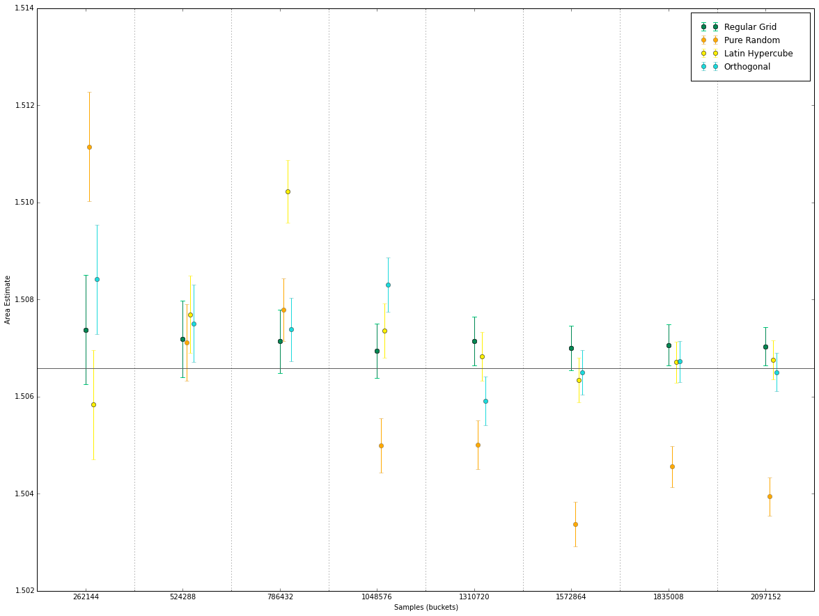
In the second experiment we will compare the methods (estimate and error) as we increase the number of samples.

Parallelism¶

We have seen that it is important, for the mean to converge to the true value and for the variance to decrease, that the samples are chosen independently. If we can generate such samples independently from eachother, we can do many membership tests in parallel. Modern GPU's (Graphics Processing Units) offer massive parallelism when a computational problem can be subdivided into relatively small and inexpensive subroutines. NVIDIA's CUDA (Compute Unified Device Architecture) is a general purpose parallel computing platform. It offers interfaces for developers to write highly parallel code to run on a CUDA Enabled GPUs.

Pixel Counting¶

In regular grid sampling, we subdivide our space $\Omega$ into cells of equal width and height and we take a single sample in the middle of the cell.

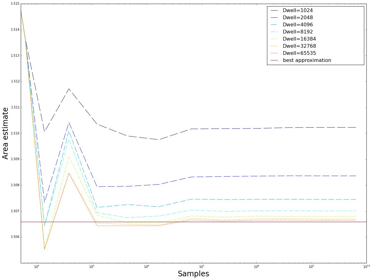
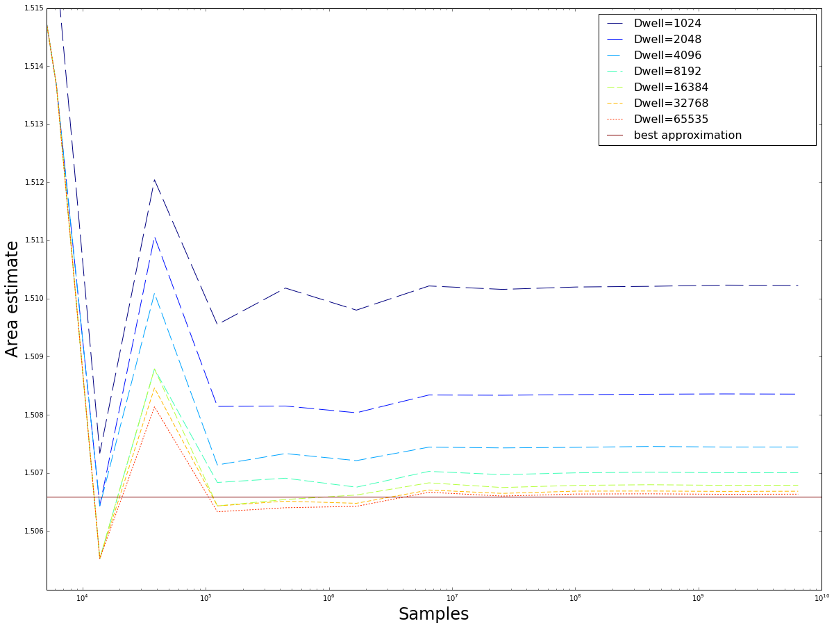
Plots of the mean value estimate for $fp32$ and $fp64$ implementations of the regular grid sampling method for an increasing number of samples up to $N\approx 0.5 * 10^10$ Note that except for some small number of values, due to using stable numerical algorithms, boths methods converge on the same values. As a reference the best estimate of F\"{o}rstemann \cite{forstemann} is used.

Performance¶

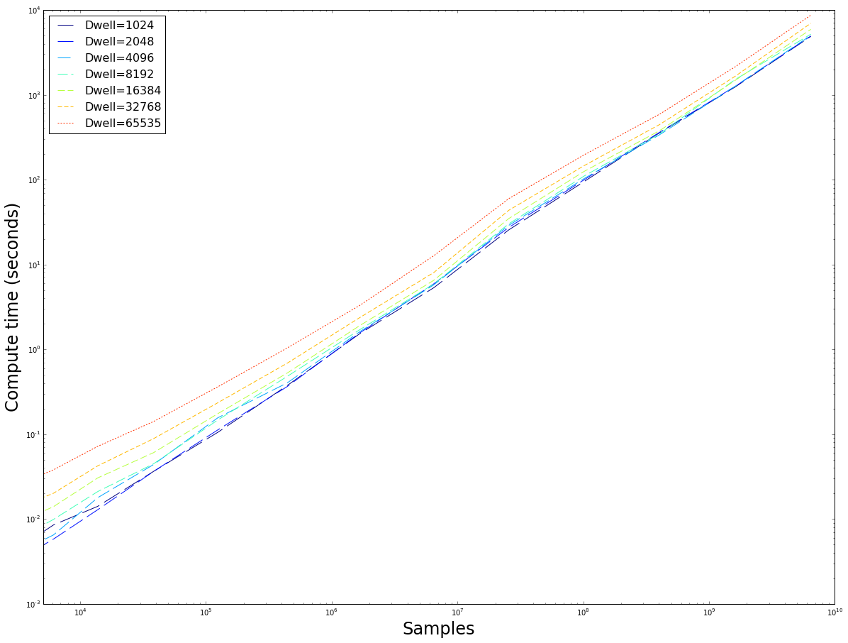
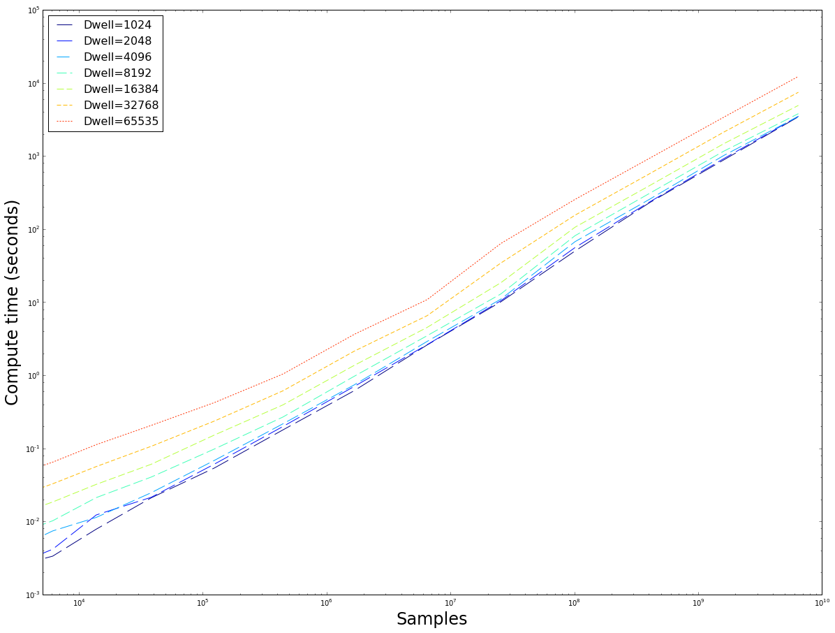
The number of samples versus the time taken to compute. Note that the computing time rapidly diverges as the maximum dwell is doubled. The $fp64$ implementation is roughly 3 times slower, whereas we have seen in figure \ref{fig:reggrid} when provided with enough samples they converge on the same values for similar dwell$_{max}$. It seems prudent to use the $fp32$ implementation because of its speed. This image also demonstrates that the method has good weak-scaling: as the input size increases, the computation time increases at roughly the same rate (linear scaling), exept for some small inputs where overhead dominates the actual computation time.

Pure Random Sampling¶

The CUDA API offers several fast pseudo-random number generators, all suitable for different purposes. We use the MRG32K3A; Multiple Recursive Generator based on the work of l'Ecuyer\cite{lecuyer}, especially suitable for stochastic simulation because of its long period $\pmb p \approx 2^{191}$. This is a pseudo-random number generator (as opposed to quasi-random). On recent hardware, it provides up to $1.2\cdot 10^{10}$ samples per second.\cite{curand}

Latin Hypercube sampling¶

Using purely random samples does not guarantee that the entire domain of the problem is covered: it is very likely that due to pure chance some areas are underrepresented in the sampling set. Using the pyDOE package \cite{pydoe} we generate a set of $N$ so-called latin-hypercube samples. In this technique, the space is divided into a $N \times N$ grid and the algorithm makes sure that each row and column are only occupied by one sample, similar to placing 8 rooks on a chessboard without two being in eachothers line of sight. This guarantees that the entire domains of the sampling area are covered.

Orthogonal sampling¶

Note that the previous method does not guarantee that the generated samples are uncorrelated. For example, all samples on the diagonal are still a valid Latin Hypercube but show a strong correlation. The pyDOE package also offers a method that generates uncorrelated samples. This method is costly: it takes us 1.3 hours to generate 2097152 samples with a correlation coefficient of 7.14227717e-04

Results¶

Experiment 1¶

Samples = 2097152 Dwell = 8192

Method	Regular	Pure Random	Latin Hypercube	Orthogonal
Mean	1.507036	1.503944	1.506755	1.506504
Variance	8.667513e-07	8.655274e-07	8.666402e-07	8.665411e-07
Error	0.001255	0.001253	0.001255	0.001254
Generate$^1$	0 s	$3.410^{-4}$s	5.4 s	1.3 h

Table: The results for Experiment 1. Note that the variances are similar, and therefore the standard errors are similar too. $^1$ the time taken to generate the samples. Generating the samples for the regular grid is taken to be zero, because calculating the sample for CUDA thread $(block, grid) = (blockID, gridID)$, and therefore requires no additional operations.

Experiment 2¶

We test the methods for increasing numbers of samples: $S=[256, 512, 768, 1024, 1280, 1536, 1792, 2048] \times 1024$

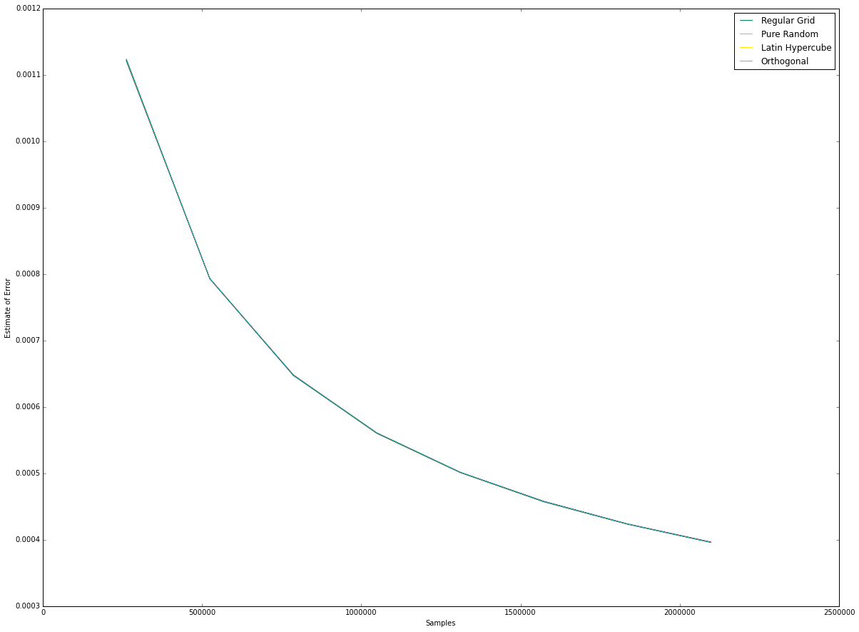
(left) The error bars for the different number of samples, for equal dwell.

(right) The errors are nearly identical and decrease asymptotically to zero, confirming what we derived in \nameref{eq:error}

Future Work¶

Pseudo- and Quasi- Random Number Generators¶

The CUDA framework offers more than one random number generator. For example, it also offers the _quasi-_random number generator based on Sobol sequences. I did not have the time to investigate all these and therefore I can not test whether naively using a Sobol sequence would perform better than any of the methods mentioned in this assignment. Since sampling a regular grid performed much better on this particular problem than RNG based methods, this is not a high priority.

Adaptive Grid¶

The device used in this assignment has compute capability 2.1. More modern devices do not only have many more cores (3072 CUDA cores vs 96 cores in the 630m), but they also offer more options. Recent devices (compute capability 5.0 and up) offer the option to launch threads from inside another thread. This could be used to adaptively refine grid cells in the Regular Grid method, using the Mariani-Silver Algorithm \cite{adinetz}

Appendix¶

Lemniscate 3¶

\label{App:AppendixA}

$$ L_3(c) ^2 =((c^2 + c)^2 + c)^2 = (((a^2 - b^2) + a) + ((2ab) + b)i)^2 + (a+bi) = a + i b + (a + a^2 - b^2 + i (b + 2 a b))^2 = r_{max}^2 $$$$ a + a^2 + 2 a^3 + a^4 - b^2 - 6 a b^2 - 6 a^2 b^2 + b^4 + i(b + 2 a b + 6 a^2 b + 4 a^3 b - 2 b^3 - 4 a b^3) = r_{max}^2 $$$$ (a + a^2 + 2 a^3 + a^4 - b^2 - 6 a b^2 - 6 a^2 b^2 + b^4)^2 + (b + 2 a b + 6 a^2 b + 4 a^3 b - 2 b^3 - 4 a b^3)^2 = r_{max}^2 $$

when b=0, we have values:

$$a = -2, \frac{\sqrt[3]{\frac{1}{2} (9+\sqrt{93}) }}{3^{2/3}} - \sqrt[3]{\frac{2}{3(9+\sqrt{93})}}, b = 0$$\begin{multline} \frac{\partial}{\partial a} (a + a^2 + 2 a^3 + a^4 - b^2 - 6 a b^2 - 6 a^2 b^2 + b^4)^2 + (b + 2 a b + 6 a^2 b + 4 a^3 b - 2 b^3 - 4 a b^3)^2= \\ 2(12 a^2 b+12 a b-4 b^3+2 b) (4 a^3 b+6 a^2 b-4 a b^3+2 a b-2 b^3+b)\\ +2(4 a^3+6 a^2-12 a b^2+2 a-6 b^2+1) (a^4+2 a^3-6 a^2 b^2+a^2-6 a b^2+a+b^4-b^2) \end{multline}

Out of two roots found using a computer algebra system, we select the root that gives us the largest value for $b$ in the dynamic plane. (Wolfram Alpha \cite{wolfram}).

A numerical approximation for the root is: $\dot{a}\approx -0.128196764513246583781488113$. This gives us extremal values:$ \dot{b}\approx \pm 1.18024821670120439545506898$. Checking higher order derivatives using the CAS reveals these are extrema and not points of inflection.